


Note: 3D graphics powered by the jsc3d project under the terms of the MIT license.

Design in 3D is not only a new paradigm, but it also requires a new set of software tools. Here is a collection of AutoLisp and VBA routines to assist the avid 3D developer. In downloading these apps, you agree with all of the Terms and Conditions presented herein and accept full liability and responsibility for their use. It is strongly recommended that you thoroughly review and test them and understand their operation before use.
To run VBA within AutoCad, you must first install the Microsoft Visual Basic for Applications Module by clicking here and following the instructions. In addition, a reference to the Excel Object Library must be added to the VBAIDE. Simply click Tools, then References, and scroll down and click Microsoft Excel XX.X Object Library.
I have also included a few of my favorite programs that you might find useful.

Bill of Materials (BOM)[Get the Sofware] [View Sample]
An essential part of the overall design is the ability to generate a detailed Bill of Materials. 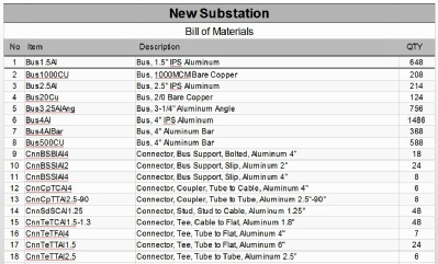 This not only assures an accurate estimate of the cost of the installation but also a check against the material supplier. With a 2D design, this involved a tedious count of materials based upon the plan and elevation views. The probability of not getting a 100% accurate count is practically assured.
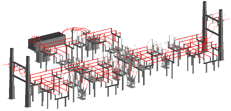
A major advantage of 3D design is that ALL materials will be included in the basic drawing. This makes the solution amenable to an automated solution. BOM creates a Bill of Material for the following and outputs the results to an Excel worksheet:
- All relevant blocks. These include all blocks from the hardware utility boxes and does not include blocks such as titleblock or ad hoc blocks.
- All footings nested one level deep within Structure and Major Equipment blocks. The _Ftg blocks are 1X1 blocks that are scaled in the X and Y ScaleFactors to represent the estimated size of the footing.
- Total lengths of all lines, polylines, arcs and splines on the Bus layers by bus type. For the BOM program to correctly determine the bus lengths, the bus path must be drawn on a layer named XBusxxxxx where xxxxx represents the bus size and type. For instance, for a 2” Aluminum bus, the layer should be named XBus2Al. If you wish to change this standard format, you will need to make the appropriate changes to BOM and other programs that rely on this format.

Bus & Jumper Routines [Get the Software]
To depict round bus and conductor in 3D, you need to display them as a round 3D object. You might first think that a wide Pline would work; however, the width is only in the XY plane and, when seen on edge, becomes a thin line. There are a number of ways to give 2D objects a third dimension. Common commands for closed 2D geometrical objects are Extrude (which adds a thickness to the 2D object) and Loft (which adds thickness and intersects two or more cross sections). For round bus, the preferred command is the Sweep command. A path, 2D or 3D, is created using Lines, Arcs, Polylines, Ellipses and Splines. The Sweep is effected by creating a circle of the desired diameter and “sweeping” it along the path. This process can be very tedious.
The following are several Autolisp routines that can assist with this process. They all use a common function, makebus, that executes the Sweep command. Within this routine are two defined list -
You can change this bus layer format, but see the caveat in the BOM routine.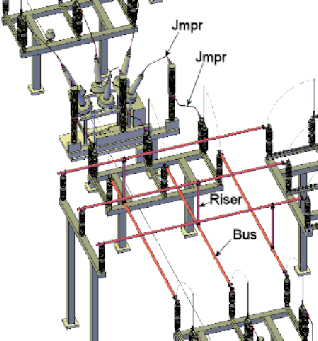
Bus -
Riser -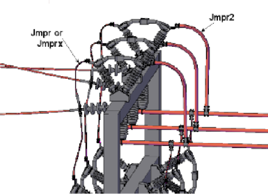 different elevations. This is a vertical riser, hence the name.
Jmpr -
Jmpr2 -
Jmpr15 -
JmprX -
LTP -
Block Manipulation [Get the Software]
The following programs manipulate blocks in various manners.
Blkupd -
Blkrep -
Blkrot -
Sag and Pole (This program has been replaced by the PSSAG program. Click here.)
Sag -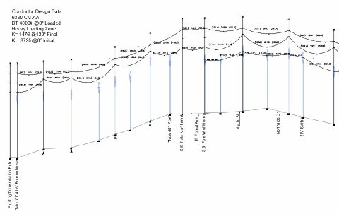 AutoLisp program for drawing a catenary curve. It was immediately evident that this program filled a gaping hole in the electric utility application. The program presented here has been adapted to make the input more functional. The required input data is:
Horizontal scale -
Vertical scale -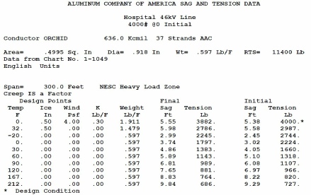 should enter 20 for the vertical (assuming a 10:1 ratio). If you enter 1 for the horizontal scale, enter 0.1 for the vertical.
K value -
Output -
Pole -
Conductor spacing -
Horizontal/Vertical Scale Ratio -
Pole height -
The user should remember that the spotting of poles and determination of conductor clearance is only a portion of the overall design process. The designer should also consider all NESC requirements for mechanical and electrical design.

Substation Design Data -
- Bus and conductor ampacities.
- Maximum allowable bus spans.
- NEMA clearances.
- Physical and electrical properties for copper and aluminum bus and conductor types.
- Bus maximum span and deflection calculator.

Pole Line Design -
- Maximum span limited by transverse wind load.
- Maximum unguyed span at line angle.
- Insulator swing angle.
- Vertical loading for running angle, multiple deadends and single deadend.
The calculations include provisions for single and double transmission circuits and single and double distribution circuits. Wire data is included for a large selection of AA and ACSR conductors and steel strand.
 Links to other resources:
- The RUS Design Guide for Rural Substations is concise reference for substation design.
- PJM Interconnection is a regional transmission organization (RTO) that coordinates the movement of wholesale electricity in all or parts of Delaware, Illinois, Indiana, Kentucky, Maryland, Michigan, New Jersey, North Carolina, Ohio, Pennsylvania, Tennessee, Virginia, West Virginia and the District of Columbia. For a wealth of information, click here.
- For their spreadsheet for calculating Outdoor Substation Conductor Ratings, click here to download spreadsheet.
- For their spreadsheet for calculating Bare Overhead Transmission Conductor Ratings, click here to download spreadsheet.
- For a copy of the Anderson Technical Data, an old and venerable reference, click here. If you can’t find the information anywhere else, you can find it here. Anderson is a part of Hubbell Power Systems, Inc.
- The RUS Design Manual for High Voltage Transmission Lines is a must read for a novice or advanced design engineer. It will give further insight to the catenary curve.
- Electrical Engineering Portal -
EEP contains a plethora of engineering information including technical articles, engineering guides and specialized Excel spreadsheets that addresses a wide range of electrical engineering specialties. As always, review in detail and understand the technical basis before utilizing any spreadsheets. To access the EEP, click here.


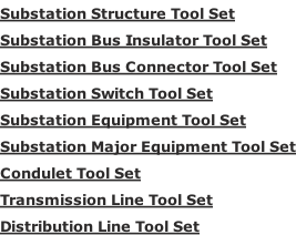
Software Toolbox